Segmentation

Segmentation is the most detailed image task: instead of a box, it labels every pixel, outlining the exact shape of objects or regions. It matters in African work wherever a precise area or boundary is the point, such as measuring the exact extent of a crop field, delineating a lesion in a medical scan, or mapping land cover from satellite imagery.

What the data looks like

A segmentation dataset pairs images with pixel-level masks. Semantic segmentation labels every pixel by class without separating individual objects, while instance segmentation also tells apart one object from another of the same class. The data is dominated by the same high-value African domains, with crop-field boundary sets like LacunaLabels and land-cover sets like LandCoverNet built because precise African-landscape masks did not exist. Satellite segmentation carries its own difficulty, cloud cover, which leaves gaps that are often filled by combining optical with radar imagery.

A mask is usually stored as a PNG the same size as the image, where each pixel value is a class id, paired with a small mapping from id to class name:

field_0007.jpg          # the image
field_0007_mask.png     # same width and height; pixel value = class id

# class mapping (e.g. classes.json)
{"0": "background", "1": "crop_field", "2": "water", "3": "built_up"}

Storing the mask as a single-channel id map, rather than a colour image, keeps it exact: a colour PNG can be re-compressed and shift a pixel's value, which silently changes its class, while an id map stays faithful to what the annotator drew.

Annotation and evaluation

Pixel-level annotation is the most expensive labelling in this playbook, so design it to be feasible: use tools with smart boundary assistance, define exactly how to treat ambiguous edges and mixed pixels, and pilot to measure how long a mask really takes before committing a budget. Because masks are so detailed, agreement is best measured by overlap rather than exact match. Segmentation is evaluated with mean Intersection over Union (mIoU), and with the Dice coefficient or pixel accuracy, all of which compare predicted masks to reference masks by how much they overlap rather than demanding identical pixels.

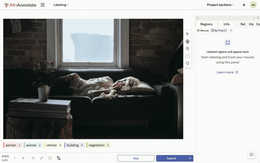
The labeling config gives the annotator a brush to paint each class onto the image:

<View>
  <Image name="image" value="$image"/>
  <BrushLabels name="mask" toName="image">
    <Label value="Crop field" background="#1F5B3F"/>
    <Label value="Water"      background="#13A4B4"/>
    <Label value="Built-up"   background="#C66A3D"/>
  </BrushLabels>
</View>

Both metrics are short to compute directly from the id-map masks, and computing them per class is what keeps a small but important region honest:

import numpy as np

def per_class_iou(pred: np.ndarray, true: np.ndarray, class_id: int) -> float:
    p, t = (pred == class_id), (true == class_id)
    union = (p | t).sum()
    return (p & t).sum() / union if union else float("nan")

def per_class_dice(pred: np.ndarray, true: np.ndarray, class_id: int) -> float:
    p, t = (pred == class_id), (true == class_id)
    denom = p.sum() + t.sum()
    return 2 * (p & t).sum() / denom if denom else float("nan")

classes = {1: "crop_field", 2: "water", 3: "built_up"}
ious = {name: per_class_iou(pred_mask, true_mask, cid)
        for cid, name in classes.items()}
print("per-class IoU:", {k: round(v, 3) for k, v in ious.items()})
print("mIoU:", round(np.nanmean(list(ious.values())), 3))

Averaging IoU across classes rather than across pixels is the deliberate choice: a thin feature like a river covers few pixels, so a pixel-weighted score would let a model ignore it entirely while still looking accurate, whereas per-class mIoU makes that failure visible.

Tracing a polygon and painting a brush mask in AfriAnnotate: